Analysing Projects

We make play evaluations for many reasons – the main one is to show spatially where the best remaining potential remains for a play using well established play mapping techniques. The other main analysis that is delivered is a calibration of success rates and volumes which is done to estimate or calibrate expected or known/mapped prospects within the play. The calibration of a Pg/POS/COS for a prospect in many companies is done by or for “the peer review process” where a group of geologists discuss various estimates for the prospects risks and the inputs into a Monte Carlo volumetric estimate to come up with a “sanctioned”/reviewed estimate of the potential of that prospect. While this process is superior to a geologist deciding on their risks and volumes in isolation the peer review process has many problems which are familiar to any geologist who has had to manage the process and the resulting database in a large company.  These problems include…

1. The same prospect if reviewed by the same peer review team at different times will come up with different estimates.
2. Different review teams looking at the same prospect at the same time will frequently make different estimates for the same prospect.
3. The presence of a senior manager with a vested interest in a positive evaluation result will distort the estimates

These issues can all be summarized under the “consistency” label so many companies have large manuals and strong processes that are enforced to minimise these complex issues.

The logic applied in these peer reviews is that a calibration of historical success rates can help constrain the evaluations for undrilled prospects which is fine in principal but in many cases the analysis is flawed. We describe the main pitfalls below and the way in which Player attempts to manage these issues and provide a better calibration of success rates and volumes for your undrilled prospects.

In many companies the total number of discoveries in a basin is divided by the number of exploration wells to come up with a basin exploration success rate which is then used to imply an average prospect risk for undrilled features. This number is typically useless and often misleading for calibrating prospects for a number of reasons the main ones being…

Pitfall Number One- The incorrect counting of exploration wells:

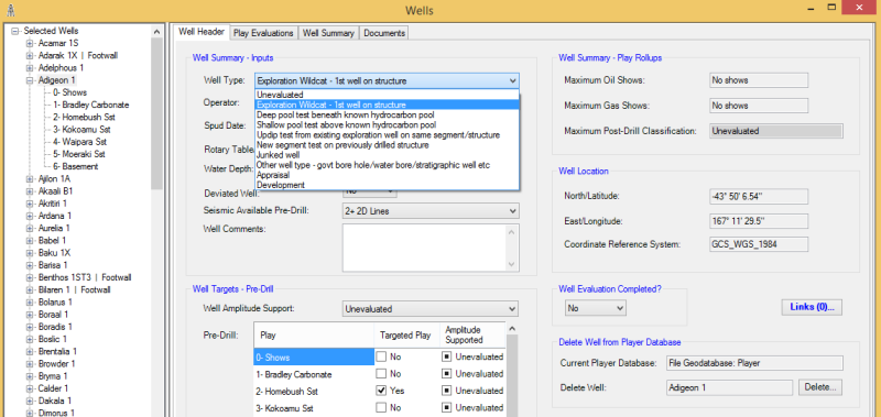
The correct definition of which wells were actually exploration wells is a common problem given that in many countries the “exploration” well type classification is attached to appraisal or development wells so that license commitments can be met.  Additionally, development wells sometimes have genuine exploration objectives – both of these variants plus the normal confusion about how to count sidetracks and/or junked wells or repeated sections in thrust belts causes uncertainty and confusion as to what the actual exploration well count is. Player enables users to modify and change classifications and then decide which well types to include in an analysis.

See Figure 1 below showing the easy to use drop down to change a vendor well classification to a user-defined option:

Pitfall Number Two- the incorrect counting of discovery wells:

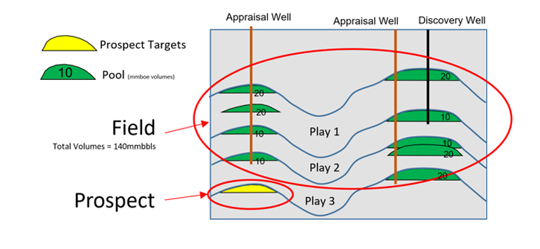
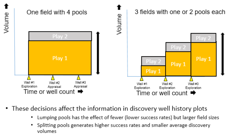
The correct definition and count of discovery wells is another common point of confusion.  The confusion arises from lateral, deeper or shallow discoveries that post-date an original discovery well.  In these cases the volumes discovered by these wells are linked to the arbitrary definition of what constitutes the field. Player allows the user to both input company estimates of volumes, which are typically better than the vendor/scout estimates, and it allows the user to specifically attribute a discovery volume to each discovery well. This sounds simple but the classification has a direct impact on the success rate and average volumes that are calculated from the analysis.                                          As shown in Figures 2 & 3 below:

Pitfall Number Three- Calculating the average success rate over an unrealistic time period:

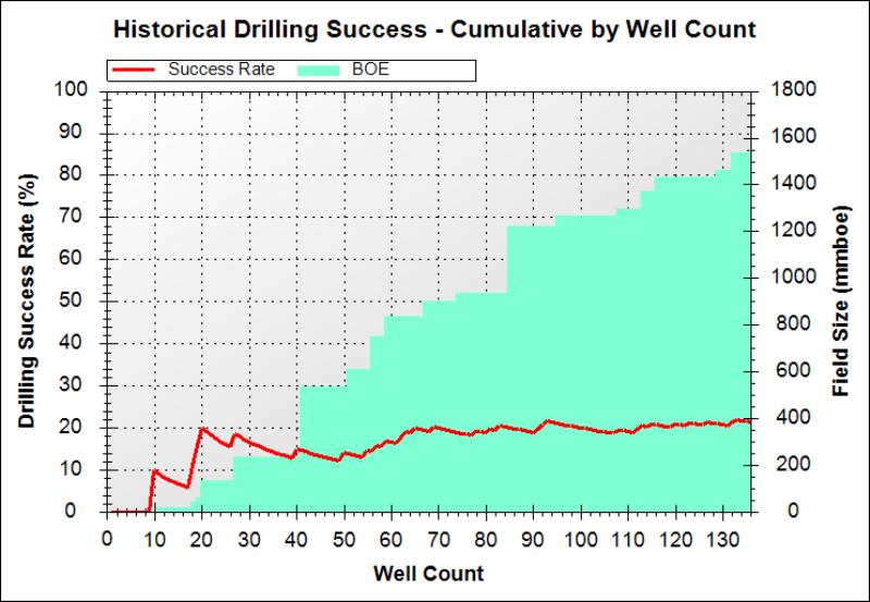
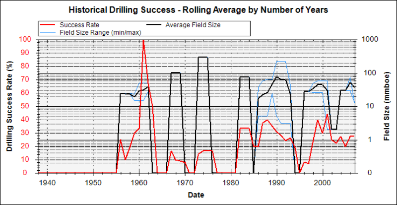
Most people when they have QC’d and edited the well and discovery datasets quote an average success rate over the entire exploration record.  However,  the better way of displaying these data is to show a 3 year (or 5 year) rolling average which highlights the more recent success rates and volumes which have been delivered by the industry.  If you know nothing else then assuming the arena is competitive and similar technology is being applied over the calibration area then the average success rate and volumes is an indication at a basin level of what your future exploration results might find on average.  Figure 4a below shows a cumulative exploration success rate through time (red curve) vs. Figure 4b which shows the 3 year rolling average of the same data! (red curve)… The latter plot gives much better insight into what your prospects may deliver.

Flaw number Four- The well success rates are calculated over an inappropriate area:

In many basins there are proven kitchen/charge areas and unproven area and an average success rate for a basin will mix up the two areas.  See Figure 5 below:

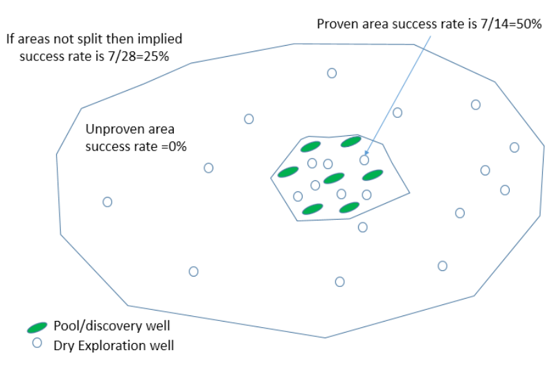
The better way of looking at success rates is to take the proven area polygon and look at the success rates in this area – the 3-5year rolling average and discovery sizes will give you an indication as to the likely future success rate in this area (if you are chasing the same trap types as the past)  – the area beyond the proven charge limits by definition has a zero success rate and in this area an extension of the proven charge cell is required or a new kitchen is needed. Regardless of the details, average success rates should NOT be basin wide estimates as these give pessimistic success rates in proven areas and unrealistic success rates in unproven areas.

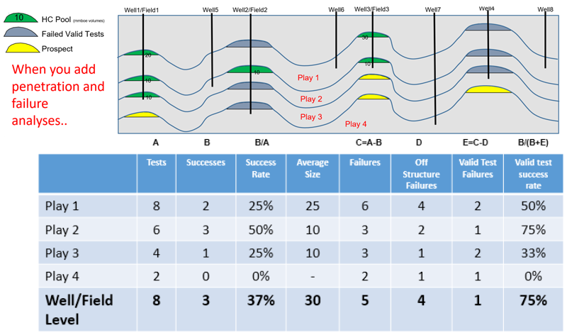
These 4 major pitfalls in success rate calibrations are all significant but even as a user if you account for all issues and look at the future success rate in a proven charge cell and look at the 3-5 year rolling average for volumes and success rates this is STILL not a calibration that can be directly applied to your prospects. To do this you have to look at play by play data which is where the well post mortem and penetration data is used which is summarized on the wonderwall plots. In simple terms a basin might have 10 wells and 2 discoveries with an average success rate of 20% but if these discoveries are both the only penetrations of a deeper play then that play has a 100% success rate and all the other plays have a 0% success rate! You need penetration and play test data to get these stats and Player collects these data in a structured orderly way and this data does not exist in the vendor datasets you can buy.

An example of this critical difference between well success and play success is shown in Figure 6 below:

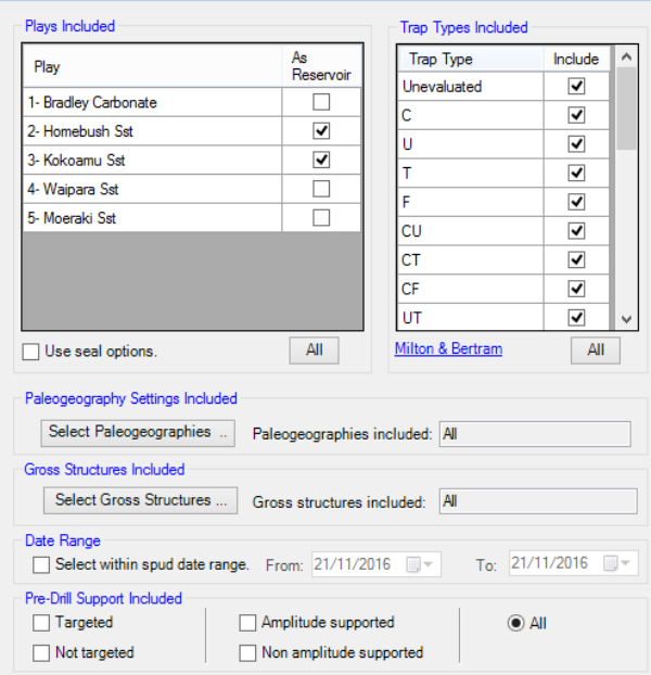
At the play by play analysis level of success rates and discovery volumes it is possible to select any combination of the following elements:

• Area – the area of the data analysis is often restricted by play or permit/license/country boundaries
• Play interval – the user can select well penetration and failure elements by one or many play intervals
• Trap type – the user can select wells that have tested different kinds of user defined traps (eg. tilted fault blocks vs reefal build-ups etc.) and can also subset the data based on which ones tested fault independent or fault dependent trap configurations
• Facies – Paleogeographic / Gross depositional environment maps can be included into the Player project
• Time interval – users can restrict their analysis by a defined time range for the exploration wells
• Pre-drill target or not?  Users can identify which plays were pre-drill targets and then do success rate and discovery volume analyses on just this subset – this analysis also clearly identifies the serendipitous discoveries which has many uses
• Pre-drill amplitudes present?  Many wells in modern exploration are based on seismic anomalies and Player offers the opportunity to look at discovery data for just these amplitude supported tests – the reality of this exploration in many mature basins is that amplitude supported exploration does NOT increase the success rate because in many basins the amplitudes are NOT direct hydrocarbon indicators. This data classification enables the lookback data to be collated quickly without analyzing every amplitude in detail (which is best done in other software packages).

It would be theoretically possible to look at the success rate and discovery volumes for the Middle Miocene tests in the Alpha sub-basin that were drilled in the 1990’s on turtle structures that intersected basin floor sands that were pre-drill amplitude supported targets! Clearly this extreme case is unlikely but in different basins there will be different subsets of data and analysis that will give the explorer insight and help calibrate the real prospects present. The interface in Player that allows a user to subset their analysis by the subsets or a combination of subsets is shown in Figure 7 below:

Importantly this analysis will also tell you what has NOT been tested since in mature basins the main game is finding complex/new traps in proven play areas so in these area you have to understand what has been tested to know whether your prospects are different or just another example of a trap type that has failed many times already.

Once this data has been collated at the play level it is then possible to look at the reasons for failure of this subset by reservoir , seal, trap and charge elements – this historical summary is automatically available once the post-drill analysis has been done and it indicates the main risks that probably should be reflected in your prospect evaluations.  However, there is no direct link between the analysis and the prospect risks, geologists still need to think about how the failure analysis is related to the identified prospects eg. in an area there might be many tilted fault block trap failures where juxtaposition was thought to be the dominant reason for failure – if the prospects in your area are all fault independent prospects (simple anticlines with no faults) then there is a logical reason as to why these prospects could have a significantly higher Pg than the historical failures.

So in summary peer reviews are fine if the right data has been collected and presented – which is rarely the case. Player is designed to collect and analyse these data and as new data is added the analysis can easily be updated. This helps the QC/QA of real prospect evaluations in a way that is transparent and documented. No other commercial software product which has been developed over 8 years has this level of sophistication and analysis and this is where companies can leverage off their local (basin mastery) datasets and make better business decisions than their competitors. Its not just traffic light maps and in many cases the decisions might be to not drill the well or to not farm into the block. Its about better decisions and improving the quality of these decisions over time which in smaller companies can be done by one or a smaller number of experienced individuals but in larger companies with diverse portfolios, rapidly moving staff and multiple offices it is about consistency, databases and information- which is what Player delivers like nothing else.

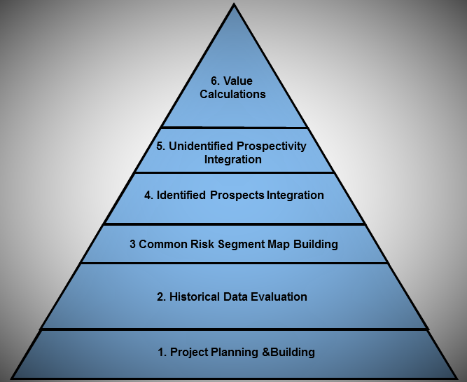
An Overview of the Analysis Process for Player Projects