Conventional vs. Unconventional Play Mapping
The Conventional Play Analysis Evaluation
Regardless of the play map type selected (either traffic light or split risking) the conventional evaluation process can be described in many ways but we like to divide it into 3 main parts:
(a) Understanding the past – understanding which plays (and trap types) have been tested, where and when?, which have worked? and why we think different plays have failed in different areas? We first of all load the discovery data into your play divisions and enable you to correct the inaccuracies and add your proprietary discovery data so you can see for each interval where the hydrocarbons are and where the wells have failed. We then evaluate the well failures using our proprietary scheme shown below:
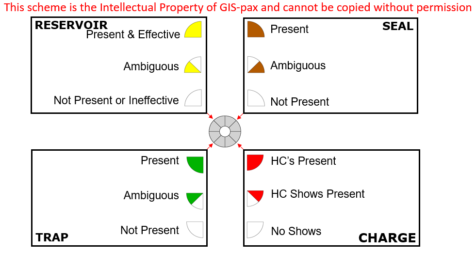
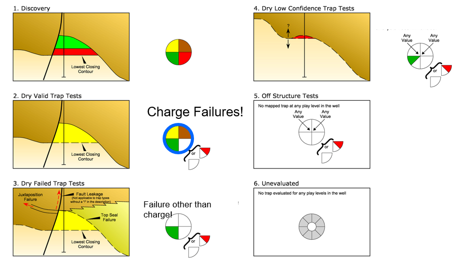
This scheme is very deliberate and powerful. This data with the penetration data is made into what we call a “wonderwall” plot to collate and show/document this critical but ever changing dataset which essentially is where you collect and save your corporate knowledge…
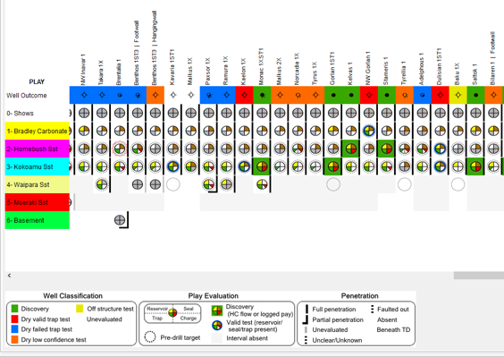
We commonly see 100’s of wells plotted out on poster sized sheets when we visit different customers. The wonderwall shows and communicates an amazing volume of exploration detail in a single format.
One of the user enhancements rolled out in 2016 is the addition of Player Docs functionality for wells, fields and prospects. An example is shown below for a well. Essentially the user collects the key maps/images/cross-sections in a powerpoint file that is viewable from within Player so when they are asked- why did you think this well failed? the key images to support their conclusion can be shown instantly. They can also be updated as information changes and all of these documents are uploaded to PlayHouse with the project data when the project is saved so that this insight is available to future users perhaps months or years later.
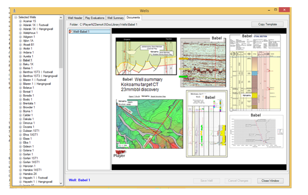
This functionality is NOT in competition with any document databases you may have in your company – you can still add hyperlinks etc as we have always offered, but as demonstrated with internal company IT changes in the past, these links sometimes do not work after various updates etc. In contrast, our key images subset will always be there- ready for you to continue your work!
Many people are intimidated by the perception of the amount of work and resources the post well analysis will take but geologists quickly learn that in basins with hundreds or even thousands of wells you can focus your efforts quickly on a selection of key wells and plays after considering the following factors
- Which are the key plays and areas you want to work/analyse? – this is normally a combination of the established plays, the plays where your company or JV has mapped leads or prospects and/or the plays that you can see are still growing (see discovery history against date by play plot below). This generally results in limited areas or subsets of blocks where you will focus your initial work…
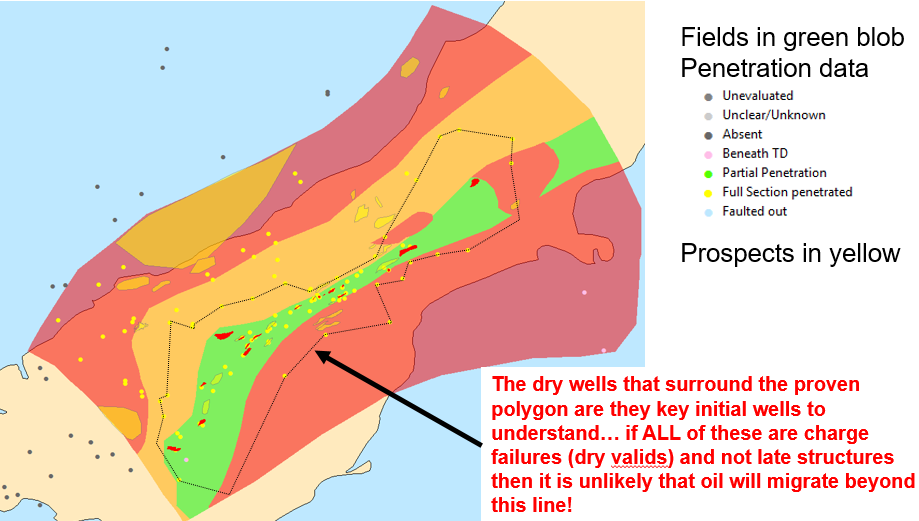
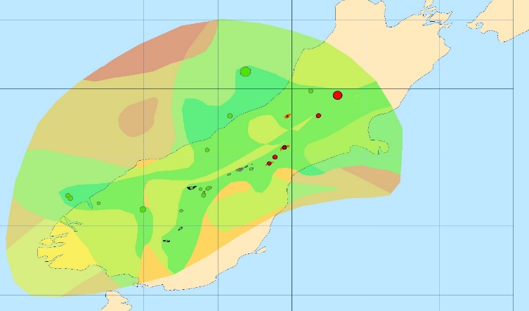
- Which are the key wells to review? – these are comprised of key stratigraphic wells that drill deep through multi-play intervals and help define the stratigraphy, wells close to or in your focus block or license areas, and wells on the “edge” of proven play areas. This latter area is particularly key since it is easy in a play to define where the pools and hence the proven play area is even without any reservoir seal or charge data. This is typically the green blob on traffic light maps and is the 100% play polygon on split risk maps. Immediately around this polygon if you have a number of wells then if they are all “dry valids” using our post well analysis nomenclature then (as long as they are not on late structures) the proven charge/play polygon is between the fields and the dry wells (as per example figure below). However, if they are all failed trap, low confidence or off structure tests then it’s possible that the play could extend over a significantly larger area. In the real world there is typically an imperfect dataset and a variety of failure types but normally you can work out which area has the best potential for a play extension.
In short, don’t try and evaluate every well and every play at the start of your evaluation. What happens in many core areas is that different blocks and plays are evaluated separately over time and eventually after a few years you will have a regional coverage and insight effectively at no additional cost. Once you have this framework, you simply add wells as they are drilled and keep your evaluations up to date.
Whatever level of analysis you do the QC of the evaluation process helps calibrate the exploration history so that meaningful plots and maps (using your corrected data) can be made that help give insight into the remaining prospectivity.
Some examples from the 30+ Player play level standard plots are shown here…
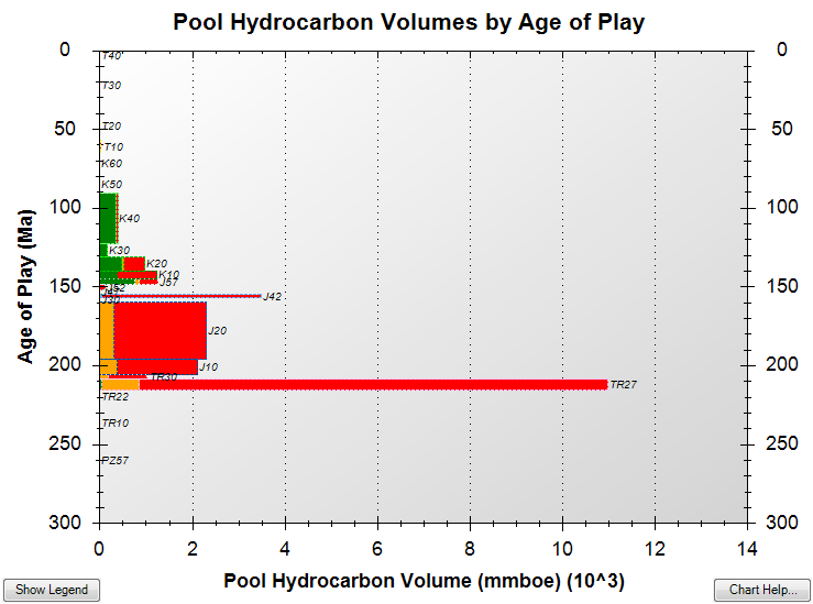
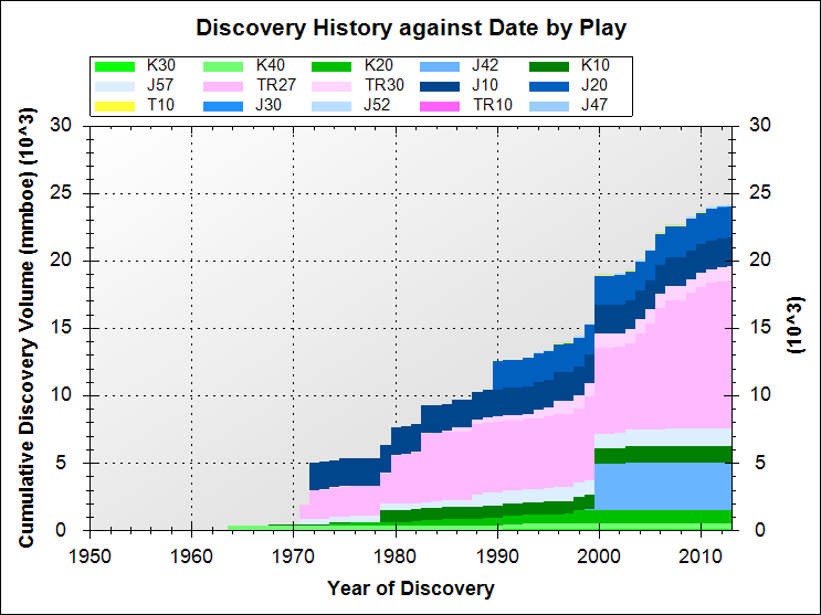
Which are the major plays? …and which ones are still “growing”?
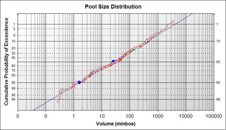
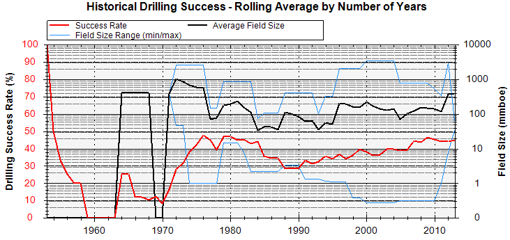
How big are the discovered pools/fields? What are the recent success rates? Discovery sizes?
This same play element data can be collected to make (well calibrated) common risk segment maps which can be convolved (stacked) into different products that highlight relative prospectivity for a play interval as shown below…
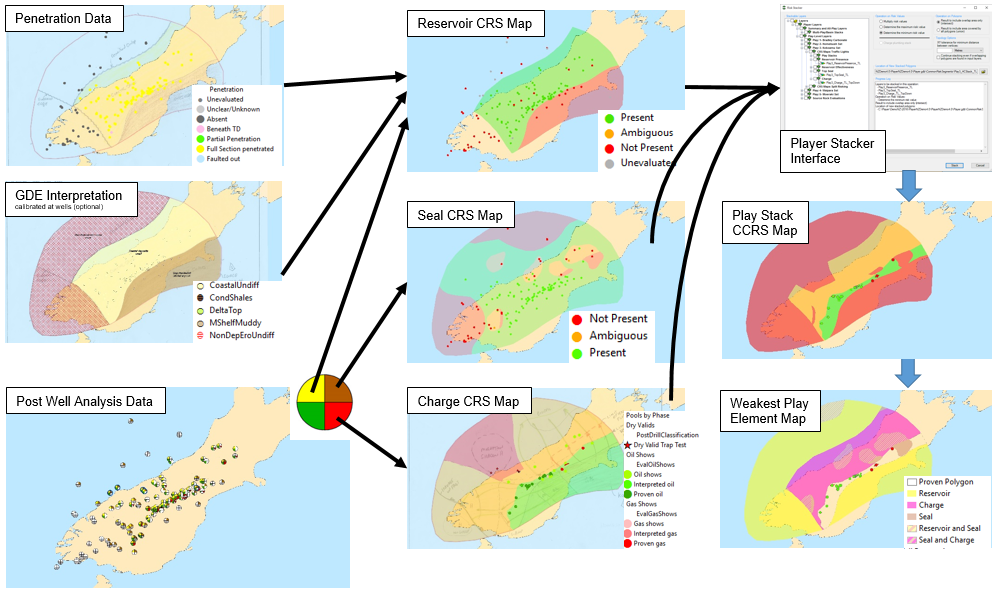
Multiple play maps can then be stacked to highlight the potential of the entire basin. We call these war maps or basin stacks and they are particularly useful for simplifying complex play analysis work into a simple output for general understanding. Shown below is a 5 play level stack where the proven areas from any play interval area shown in dark green.
(b) Quantifying the present – Collecting and evaluating both the undrilled identified leads and prospects and determining:
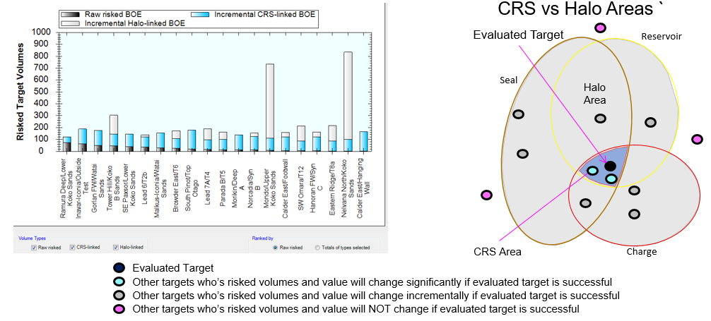
1. Which ones will de-risk entire areas or populations of prospects and which ones will have zero effect on adjacent prospects? This is where the split risk methodology shines since this approach plus Player can very quickly show the impact of success on a target by target basis. This is critical analysis because this analysis will possibly change what you drill!
2. In the proven areas where the play risks will never change with future exploration success we recommend collating trap type data for pools/discoveries, well failures and prospects so you can work out which new trap types might offer material future potential in these heavily explored areas.
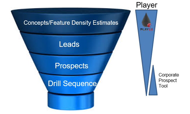
Player has been designed to quickly collect the prospectivity dataset and we are specifically not competing with detailed prospect volumetric tools which are best applied to the possible drill sequence rather than on screening level prospectivity assessments. We have built links to all the major prospect tools used in the industry today including MMRA and Geox. The concept we have is that Player and simple screening volumetric tools would be used to collect all the identified prospectivity quickly and efficiently and then in time only a subset of these will be high graded for drilling. As an industry we spend a disproportionate amount of resources making these detailed volumetric estimates since we know they will all be wrong. We think it is better to initially capture more prospects and leads quickly rather than spend a significant amount of time analysing a few that may have been arbitrarily and wrongly high-graded.
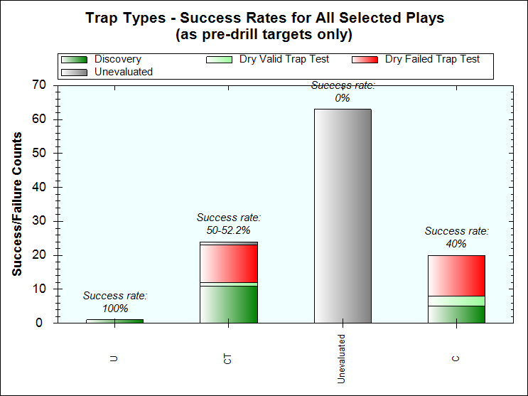
When we collect these data we can also use the collected well pool and post well analysis data to help calibrate our identified prospectivity. Specifically we can subset the exploration tests by area/polygon, play interval, trap type, facies/GDE/paleogeography, drill date, whether it was a pre-drill target, and if it was amplitude supported or not. For any such subset we can then look at the success rates and discovered volumes and compare this subset to the matching prospects.
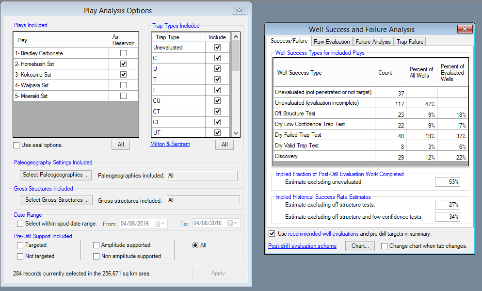
Which discovery/well/prospect subset do you want to analyse?.. then the success rate summary for this subset calibrates what the real success rate has been.
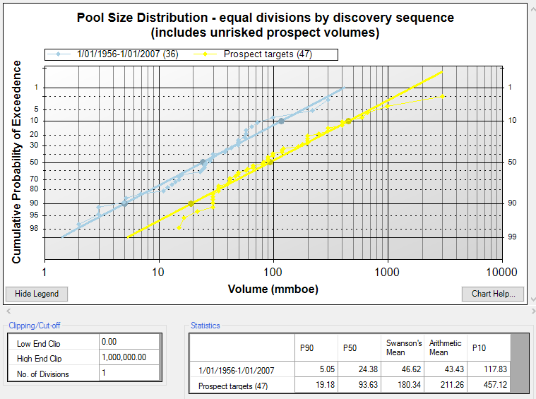
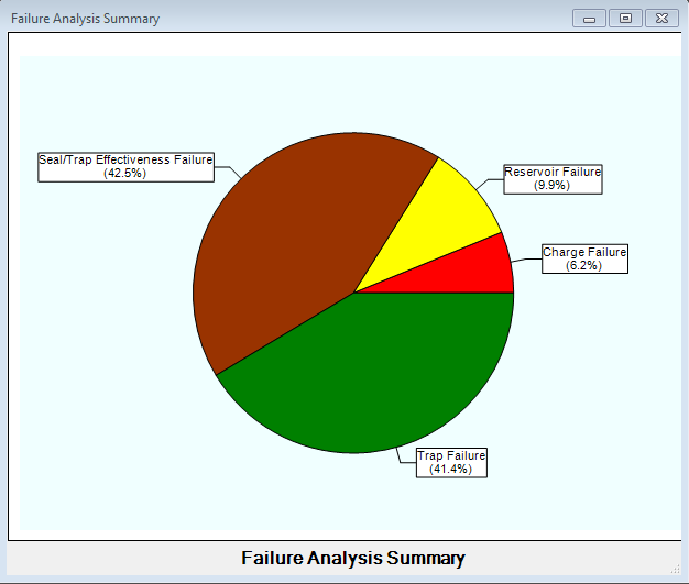
Above a comparison of the prospect volumes vs the discovered volumes for this subset and the reasons why the subset wells failed from the post well analysis data. In this example seal and trap effectiveness and trap presence look like the key risk elements and the user can check to see if these are indeed the key risks identified for the prospect subset.
This play by play data can be used to calibrate the prospects – well count data cannot be used to do this and indeed it can be very misleading – for example imagine a basin with 10 exploration wells and 2 discoveries. An inexperienced geologist might suggest a 20% success but if the 2 discoveries were the only wells to drill a particular play then the success rate for that play is 100% and the success rates for all the other play intervals are 0%! Success rates are dangerous and often misleading.
(c) Predicting the future – Once we have properly and efficiently evaluated our identified prospectivity against the historical exploration record we can turn to understanding what the future might hold. This can be done in many ways but normally it is a two step process.
The first step is to try and estimate which prospects and leads we have not included in our analysis. This may be for many reasons but normally it is because we don’t have the seismic data and/or the seismic ties to well control and/or the time to map prospects. In many white space or data lean areas we can see potential traps on loose 2D seismic grids but often we do not have sufficient data to map features. In these areas and by analogy with other similar geological areas, we can add polygon estimates (at a specific play level) of feature densities (number per 1000km2 is the normal unit) and the average size or a field size distribution of the future fields. This process is easy to do in Player but the calibration of both of these numbers is the key challenge. In the anolog/calibration area the structural density has to include the failed valid tests and prospect data in addition to the pool/field data. In the area of interest where the anolog is being applied, the drilled valid tests and the prospects have to be subtracted from the anolog feature density estimate.
When geologists use the feature density approach they typically make two technical mistakes. First, the approach is predicated on the prediction of structures based on common basement rheological responses over large areas to shared tectonic events. This means that normally large stratigraphic traps cannot be included or predicted by this methodology and the calibration and predictions should be limited to structural/tectonic features.
The second mistake is to make these predictions over proven well explored areas which contain numerous discoveries (rather than in white space areas). The reality is unless the predictions in these areas are ONLY for smaller field sizes that may not have been the focus for exploration then the estimates will be wrong. Modest to large traps next to fields get drilled quickly in the real world and these larger estimates are simply guesses and are probably wrong. In these areas you need real prospect data supplemented by a methodology to predict the small field fraction in that area. Our suggestion in these proven areas is to divide them into “simple/easy” areas (layer-cake stratigraphy, simple structures, well imaged, simple petroleum/source systems, well explored by all technology by competent companies in OECD countries etc) vs “complex/hard” areas (complex stratigraphy, complex structures, poor imaging, complex petroleum systems, inefficiently explored by various companies in countries trying to kill you etc… We call this dimension the serendipity index and the basic logic is if you have identical prospect risks and volumes in two extreme serendipity index areas then you have a better chance of getting lucky in the complex/hard one – the complexity and toughness preserves upside potential.
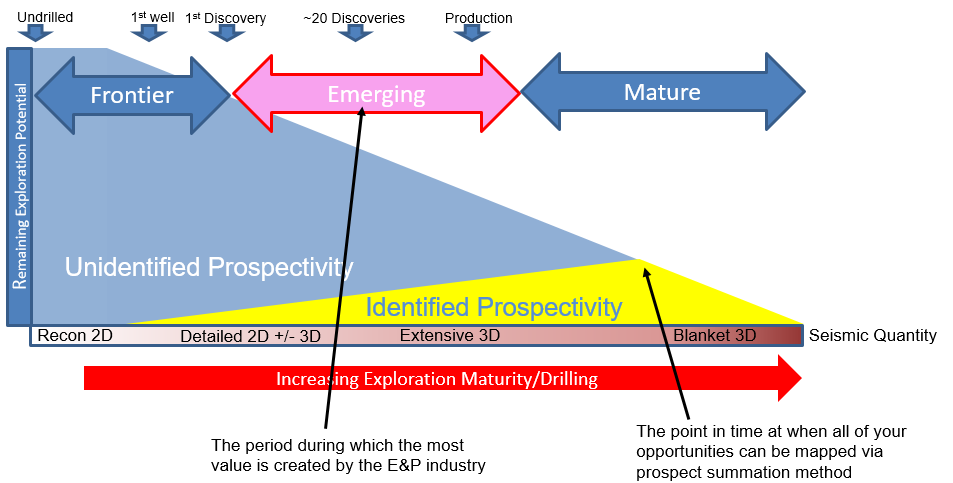
Feature density (UIP) estimates should normally be limited to frontier and emerging exploration maturity areas.
The second step in future predictions is to take our prospectivity estimates and sum them into plays and blocks. This summation into blocks is key because this is the commercial unit of currency that we deal with in exploration. This divestment and acquisition process is normally a continuous process.
The Unconventional Play Analysis Evaluation
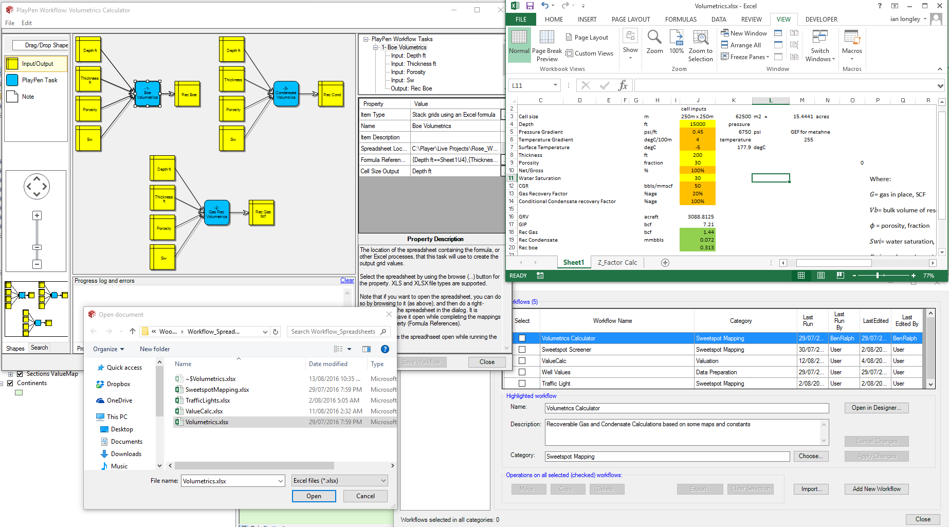
The E&P industry does not have a consensus as to how to do unconventional play assessments so the process is highly variable from company to company. In addition to this every unconventional play is subtly different from the others resulting in different geological risk elements being used for different plays. Our software solution for this world is PlayPen where we offer a series of grid/raster tools to do key analysis functions together with a workflow interface that can link grids, polygons and constants together using arcbox tools and/or excel spreadsheets. The link to excel is particularly useful for many companies because many of the evaluations of existing opportunities have already been captured in spreadsheet evaluations and PlayPen now offers the opportunity to spatialize this existing work and make heat/prospectivity maps quickly and easily.
A description of the power of PlayPen to make unconventional evaluations is shown in this sequence of images which show the following steps:
- The export of well values from Accumap and other third party providers into arcshapefiles which are then turned into a grid surface using a Playpen workflow linked to a an arc raster manipulation tool.
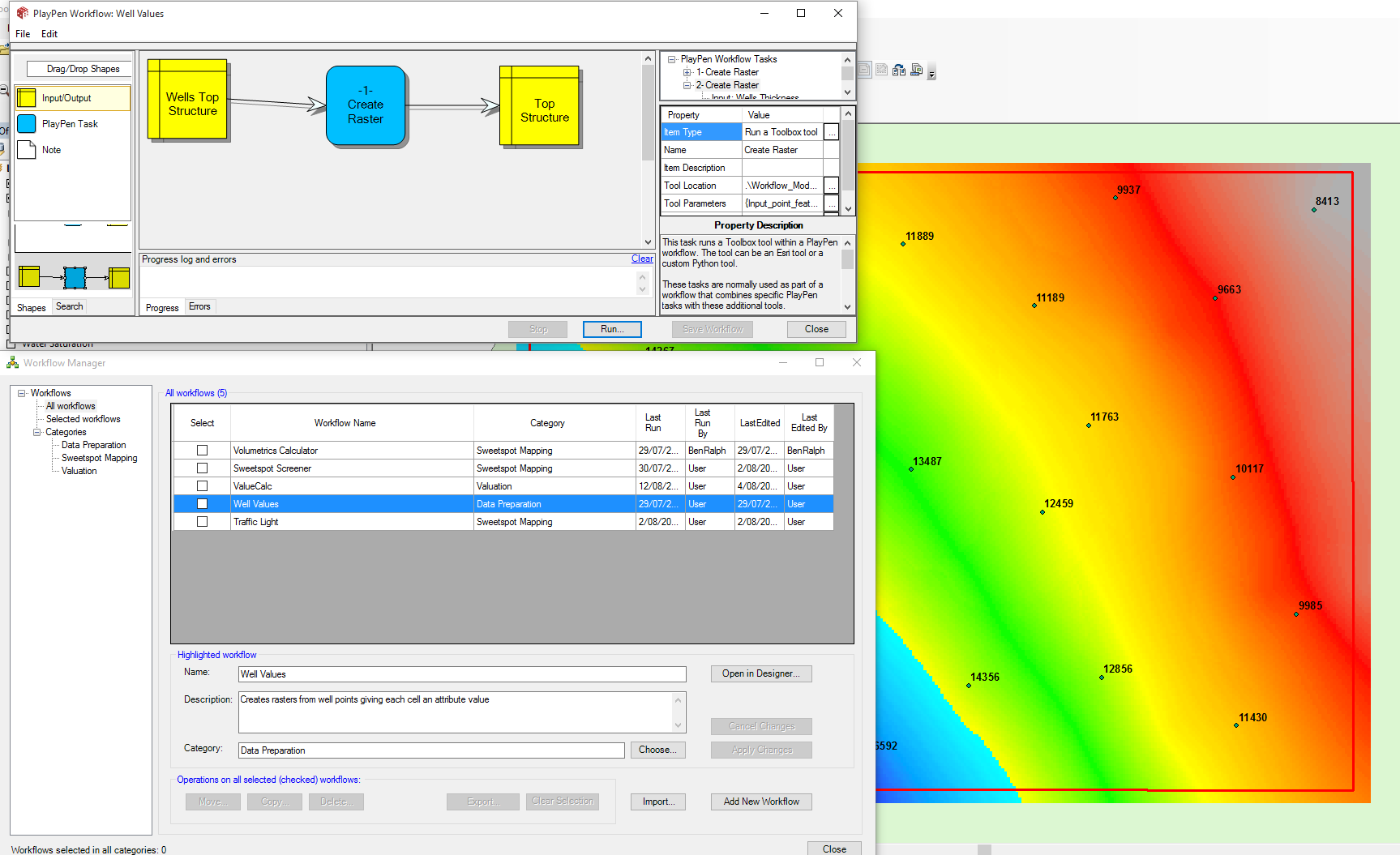
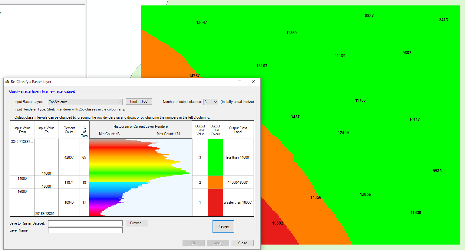
- This is done for various well elements- a PlayPen workflow is used to make various sweetspot maps – the one shown here is the traffic light variety where each element is divided into traffic light windows using the “reclassify a raster dataset” tool as shown below. The tool is pointed at the depth grid, then a histogram of the raster values as shown below is displayed and the user can select to divide this distribution into any number of divisions. In the example below, the user has divided the histogram into 3 divisions, that can then be coloured, given a value and some description, and then this output can be saved. This process is done for all the elements separately, then all of these traffic light maps are stacked.
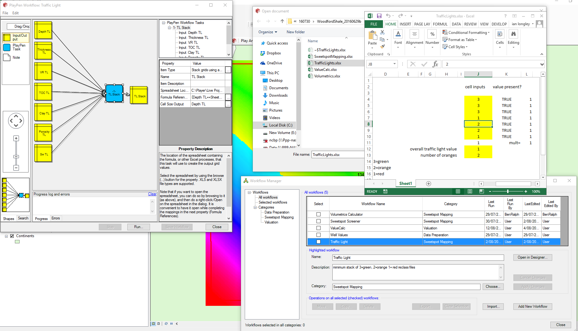
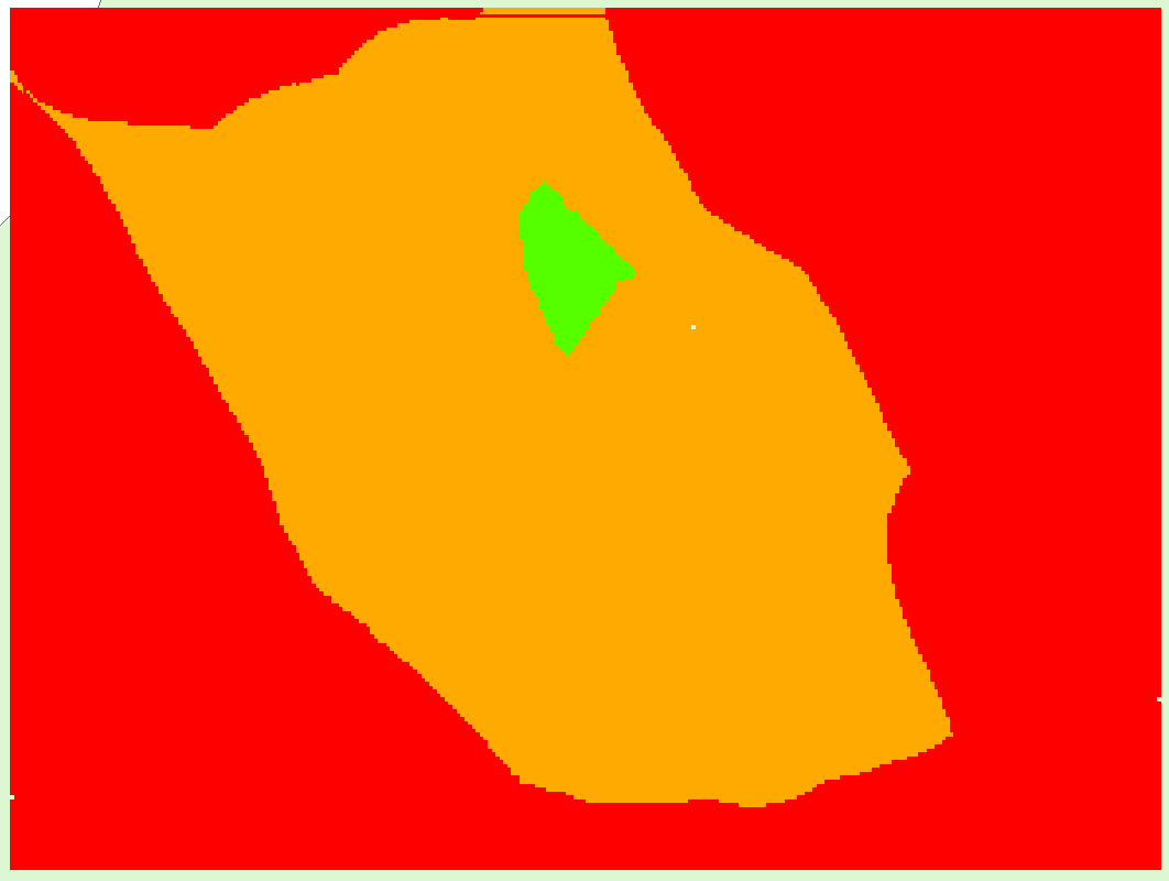
- The traffic light stack process uses a PlayPen workflow as shown below where the traffic light workflow is set up to point to all the traffic light maps which are grid node by grid node pumped through the excel spreadsheet to make a raster output making the sweetspot output map shown. This process is quick to set up and easy to modify…
- Another way of evaluating the potential of an unconventional play is to calculate “what the rocks can give us” ie. an evaluation of the ‘in place and recoverable volumes’. In this example PlayPen is used to calculate in place and recoverable volumes using constant recovery factors which in the real world would probably be well points where the recovery factor was estimated from production data decline curve analysis. In this case the gas expansion factor is calculated in each grid cell using a pressure gradient and geothermal gradient constant applied to the depth maps in excel. This GEF is complex and shows how Playpen can simplify many of these difficult estimates.
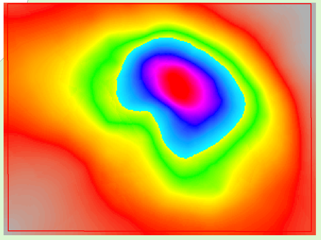
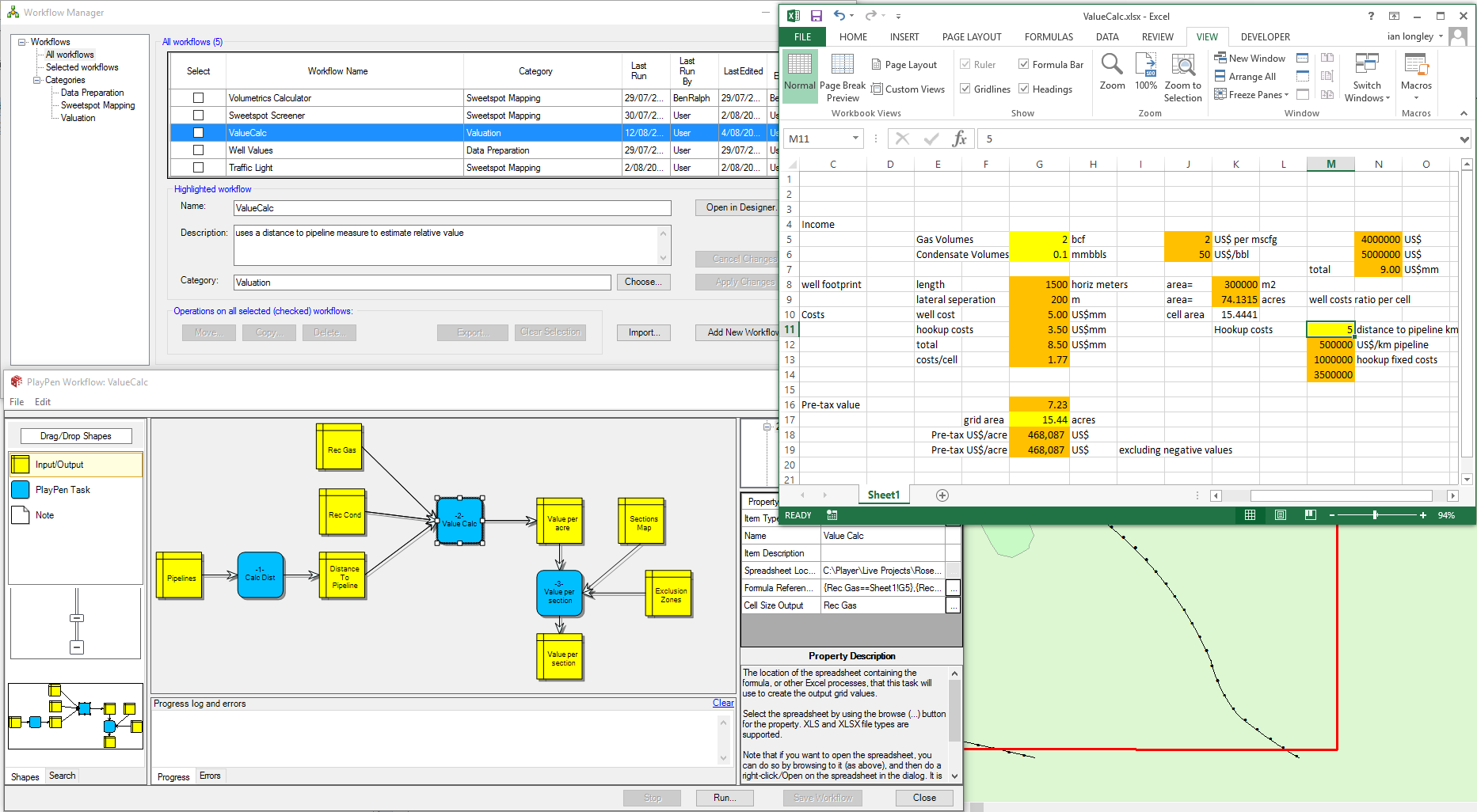
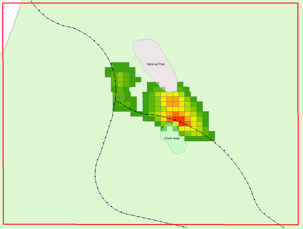
Below, we have made an example of an economic evaluation. In this case the distance to pipelines is calculated and a unit cost applied to any development tieback. This cost is added to the cost of a generic horizontal well (with an assumed spacing and drainage) and this total cost is balanced against the income generated from the recovered volumes (estimated from the “what can the rocks give us” evaluation described above). In this simple example we can calculate the value of each grid node then roll these up into the blocks so that a total value of each bid block can be estimated. The numbers are rough but the output provides a heat map that is based on user inputs and models and is the key map needed for decision making.